Dynamic Forecasted Measures - Page 2

jesse_sherb · 11-01-2018 09:06 AM

Scenario

Predictive analytics and machine learning have been popular buzzwords as of late and can provide tremendous value for organizations. But what about folks who don’t have a data science team or the resources to build out machine learning models? There is still tremendous value in being able to provide lightweight projections or linear forecasts to see how your business may be pacing through the end of the month, quarter, year, etc. Using simple modeling techniques in Looker, we can provide some baseline predictions depending on how we’re performing thus far.

Please note, this article contains the use of Looker Parameters and Liquid. Here’s some additional resources:

The Templated Filters and Parameters Docs tutorial which discusses creating the field and applying the user input.
The parameter reference page for this field type and its allowed_values subparameter
The Field Parameters page includes the parameter field type and says which LookML parameters can be subparameters of a parameter field
The Liquid Variable Reference page mentions the {% parameter %} liquid variable

The Dimension, Filter and Parameter Types page indicates which LookML type parameter values can be used with parameter fields.

Goal

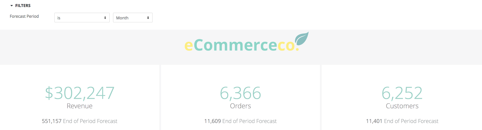
Let’s create a pattern that allows us to take a look at how we’re forecasting for any measure, for any period of time. Below is an example dashboard to illustrate.

Step 1: Create Dynamic Forecasting Timeframes

The core philosophy is to find how far along that period we are, so we can linearly forecast sales through the end of the period.

First, we need to create a parameter to give us our forecast period options. Then we’ll need to find how far along we are into the selected forecast period. For example, if today is October 18th, and we’ve selected month, we’re 18 days in. For this example, we’ll create week, month, quarter, and year. See below.

parameter: prediction_window {
    allowed_value: {
      label: "Week"
      value: "week"
    }
    allowed_value: {
      label: "Month"
      value: "month"
    }
    allowed_value: {
      label: "Quarter"
      value: "quarter"
    }
    allowed_value: {
      label: "Year"
      value: "year"
    }
    }

Now that we have our parameter which allows our users to select which time period their interested in forecasting, we’ll need to create a dimension that dynamically finds the first day of that selected period. Here’s our first use of the Liquid Variable Reference:

dimension: first_day {
    type: date
    sql: date_trunc({% parameter prediction_window %},getdate()) ;;
    convert_tz: no
  }

Next, we’ll have to find the last day of the period, so we can calculate what percentage of the period is complete, and how much we have left to go. We’ll do this with a dimension and a Liquid IF statement that leverages our prediction window parameter. If you have a more simplistic application of this in mind (for example, your prediction period is always the same), see below for examples without the use of Liquid.

  dimension: last_day {
    type: date
    sql: {% if prediction_window._parameter_value  == "'quarter'" %}
                last_day(dateadd(month,2,${first_day}))
         {% elsif prediction_window._parameter_value  == "'month'" %} 
                last_day(${first_day})
         {% elsif prediction_window._parameter_value  == "'year'" %}
                last_day(dateadd(month,11,${first_day}))
         {% elsif prediction_window._parameter_value  == "'week'" %} 
               dateadd(day,6,${first_day})
         {% endif %} ;;
    convert_tz: no
  }

  dimension: hours_since_start {
    hidden: yes
    type: number
    sql: datediff(hour,${first_day},getdate()) ;;
  }

This will calculate the number of hours into the selected time period. This is important for finding what percentage of the period has been completed, so we can forecast the remainder. It’s important to do this using hours rather than days to prevent 0% completion on the first day of a period (i.e. October 1st).

  dimension: hours_until_last_day {
    hidden: yes
    type: number
    sql: datediff(hour,getdate(),${last_day})+24 ;;
  }

We add +24 here to account for the current day. Date Diff is going to give us the difference in hours between two dates. For example, SELECT DATEDIFF(hour,'2018-10-01 00:00:00','2018-10-18 00:00:00') will give us 408 hours, or 17 days. We need to account for “today” or the 18th in this example.

Finally, we’ll bring it together to find the total hours in the period so we can complete the percentage of period calculation as seen below.

  dimension: hours_in_period {
    hidden: yes
    type: number
    sql: ${hours_since_start}+${hours_until_last_day} ;;
  }

  dimension: percentage_of_period_completed {
    type: number
    sql: 1.0*${hours_since_start}/NULLIF(${hours_in_period},0) ;;
    value_format_name: percent_2
  }

Step 2: Scale This Pattern Across Multiple Measures

In order to reuse the pattern we’re creating for multiple measures to prevent repeat code writing, we can introduce a metric selector. Below is the syntax to do so. Here, we’re leveraging these example dimensions, but these could be any fields you care about.

Sample Dimensions:

  dimension: sale_price {
    type: number
    sql: ${TABLE}.sale_price ;;
    value_format_name: usd
  }

  dimension: order_id {
    type: number
    sql: ${TABLE}.order_id ;;
  }

  dimension: user_id {
    type: number
    sql: ${TABLE}.user_id ;;
  }

Metric Selector:

 parameter: metric_selector {
    allowed_value: {
      label: "Sales Price"
      value: "total_sale_price"
    }
    allowed_value: {
      label: "Customers"
      value: "customers"
    }
    allowed_value: {
      label: "Orders"
      value: "orders"
    }
  }

  dimension: selected_metric {
    hidden: yes
    type:number
    sql: 
{% if metric_selector._parameter_value  == "'total_sale_price'" %} ${sale_price}
{% elsif metric_selector._parameter_value  == "'customers'" %}${user_id}
{% elsif metric_selector._parameter_value  == "'orders'" %} ${order_id}
{% endif %} ;;
    value_format_name: decimal_0
  }

Step 3: Apply Metric Selector to This Periods vs. Projected Period Measures

Now we have our forecast period defined as well as the metric we want. The next step is to calculate the value for the current and projected period. This will result in the following:

Up until this point, we have modeled both filter parameters and all columns except the last two. First, we’ll calculate the value of the measure for period-to-date. We’ll then divide that by the % of the period we’ve completed (i.e. October 15th is 48% through the period, or 15/31 days, 360/744 hours). This will give us the linear forecast for the entire time period. Here’s where it gets a bit tricky, see below for the syntax!

  measure: this_period_measure {
    type: number
    sql:
    {% if metric_selector._parameter_value  == "'total_sale_price'" %}
        SUM
    {% elsif metric_selector._parameter_value  == "'customers'" %}
        COUNT
    {% elsif metric_selector._parameter_value  == "'orders'" %}  
        COUNT
    {% endif %} (CASE WHEN ${created_raw} >= ${first_day} THEN ${selected_metric} END)
    ;;
    value_format_name: decimal_0
  }

You may ask yourself why we’re doing the aggregation of our dimensions (i.e. sale_price) in the “this_period_measure” instead of pointing to a measure that’s already performing the aggregation. We need to refer to dimensions in the first part of our CASE statement: CASE WHEN ${created_raw} >= ${first_day}. Therefore, we need to group by those dimensions in order to perform the aggregation. For example, CASE WHEN ${created_raw} >= ${first_day} THEN SUM(${sale_price}) will return an error. The above is a way to dynamically wrap the entire CASE statement in whichever type of aggregation is needed for our analysis.

 measure: projected_measure {
    type: number
    sql: 1.0*${this_period_measure}/NULLIF(${percentage_of_period_completed},0) ;;
    value_format_name: decimal_0
  }

For those of you working with COUNT DISTINCTS, below is the syntax for that.

measure: this_period_measure {
    type: number
    sql:
    {% if metric_selector._parameter_value  == "'total_sale_price'" %}
        SUM
    {% elsif metric_selector._parameter_value  == "'customers'" %}
        COUNT(DISTINCT
    {% elsif metric_selector._parameter_value  == "'orders'" %}
        COUNT(DISTINCT
    {% endif %} (CASE WHEN ${created_raw} >= ${first_day} THEN ${selected_metric} END)
    {% if metric_selector._parameter_value  == "'customers'" %}
        )
    {% elsif metric_selector._parameter_value  == "'orders'" %}
        )
    {% endif %}
    ;;
    value_format_name: decimal_0
  }

And for the final product:

Solution without using Parameters or Liquid:

### TIME WINDOW DIMENSIONS ###


dimension: first_day {
  type: date
  sql: date_trunc('quarter',getdate()) ;;
  convert_tz: no
}

dimension: last_day {
  type: date
  sql: last_day(dateadd(month,2,${first_day})) ;;
  convert_tz: no
}

dimension: hours_since_start {
  type: number
  sql: datediff(hour,${first_day},getdate()) ;;
}

dimension: hours_until_last_day {
  type: number
  sql: datediff(hour,getdate(),${last_day})+24 ;;
}

dimension: hours_in_period {
  type: number
  sql: ${hours_since_start}+${hours_until_last_day} ;;
}

dimension: percentage_of_period_completed {
  type: number
  sql: 1.0*${hours_since_start}/NULLIF(${hours_in_period},0) ;;
  value_format_name: percent_2
}

### THIS PERIOD AND PROJECTED PERIOD MEASURES ###


measure: this_period_measure {
  type: sum
  sql:CASE WHEN ${created_raw} >= ${first_day} THEN ${sales_price} END;;
  value_format_name: decimal_0
}

measure: projected_measure {
  type: number
  sql: 1.0*${this_period_measure}/NULLIF(${percentage_of_period_completed},0);;
  value_format_name: decimal_0
}